静态 Notebook 阅读页:展示保存的代码和输出,未重新运行。
<img src="./img/uoxf-logo.png" width="200" style="float: right; margin-left: 5%" />
Data Analysis and Statistics
Prof Adrian Oeftiger
(adrian.oeftiger@physics.ox.ac.uk)
Based on lectures given by Dr Jenny Barnes
The Scientific Method
Feynman on the Scientific Method:
"It doesn't make a difference how beautiful your guess [theory] is, <br />it doesn't make a difference how smart you are, <br />who made the guess, or what his name is...
If it disagrees with experiment, it's wrong."
\(\implies\) How can we be certain that an experiment and theory agree or disagree?
This is what we hope to teach you with this course and throughout your time in the practical course.
This course
4 lecture slots:
- 3 lectures
- problem sheet: go through questions in lecture 4
Syllabus (in Year 1 handbook)
- A-level Maths plus the bridging material in (a) data analysis and statistics and (b) computing are assumed
- Qualitative introduction explaining what experiments are, what they are used for in science, and other relevant concepts such as hypothesis or model testing
- The fundamental origins of experimental uncertainty, e.g. shot and Johnson noise
- Examples throughout the course, from contemporary physics or famous discoveries, discussing experimental design, technique, and instrumentation as well as data analysis
- Uncertainties in measurements including dominant error, random and systematic errors, accuracy and precision, derivation and use of error propagation formulae assuming independent, normally distributed errors (i.e. no covariance matrices)
- Gaussian and Poisson distributions (as the distributions found in first year practicals), central limit theorem, least squares fitting (including weighted), meaning of residuals, confidence limits, simple statistical tests
- Practical implementation of the above in software and in data presentation, including
- How to produce a plot (e.g. labels, units, title, expression of uncertainties etc.): see DA01 – Data Analysis practical
- How to describe and present a numerical answer sensibly, with appropriate precision: used in practical course
- Other useful skills in physics such as estimation. A pragmatic approach to data analysis should be stressed
This first year material is taught through (this) short lecture course and the practical work. It is continually assessed through practical work (i.e. through log book assessment, lab reports, and discussion with demonstrators).
As is usual, knowledge of the first year syllabus will be assumed in the second year, where it can be examined and/or encountered in practicals.
Recommended Books
| <a href="https://solo.bodleian.ox.ac.uk/permalink/44OXF_INST/35n82s/alma991022211321607026"><img src="./img/Hughes_Hase.jpg" alt="Measurements and Their Uncertainties: A Practical Guide to Modern Error Analysis (Ifan Hughes and Thomas Hase)" width="326" /></a> | <a href="https://solo.bodleian.ox.ac.uk/permalink/44OXF_INST/35n82s/alma991014695729707026"><img src="./img/Vaughan.jpg" alt="Scientific inference: learning from data (Simon Vaughan)" width="300" /></a> |
|---|---|
| <a href="https://solo.bodleian.ox.ac.uk/permalink/44OXF_INST/35n82s/alma991022211321607026"><img src="./img/qr-code-measurement-uncertainties.png" alt="QR code for Measurements and their uncertainties book" width="100" style="margin: auto;" /></a> | <a href="https://solo.bodleian.ox.ac.uk/permalink/44OXF_INST/35n82s/alma991014695729707026"><img src="./img/qr-code-scientific-inference.png" alt="QR code for Scientific inference book" width="100" style="margin: auto;" /></a> |
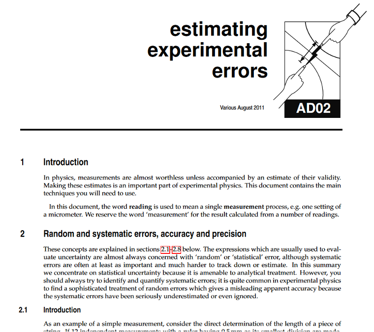
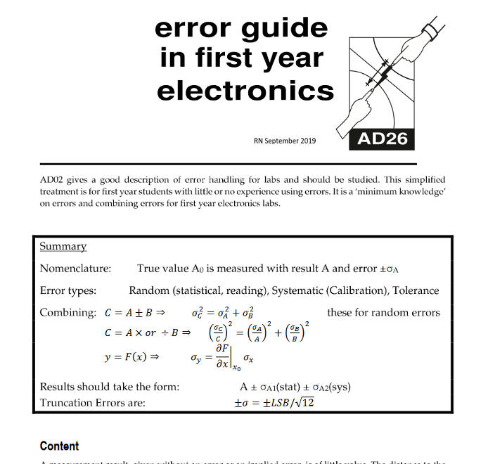
Useful documents
 |
 |
|---|
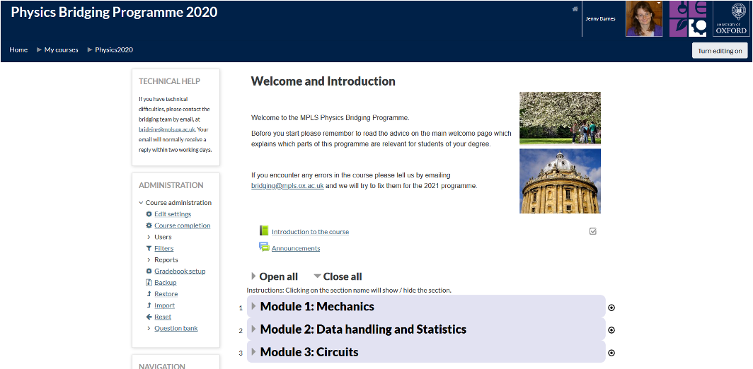
Material on MPLS bridging programme
Web address: https://mplsbridging.conted.ox.ac.uk/
You should have been sent a username and password over the summer, if not contact bridging@mpls.ox.ac.uk .
 |
 |
|---|
Other resources
Try the “More or Less” podcasts on Radio 4, available through BBC sounds app or at: https://www.bbc.co.uk/sounds/brand/b006qshd
Online statistics resources can be found at: http://www.statstutor.ac.uk/
A very helpful leaflet summarising lots of statistics formulae can be found at: https://www.statstutor.ac.uk/resources/uploaded/43799-prob-stats-ff-for-web.pdf
DA01 – Basic Data Analysis in Python
This is a practical which teaches you:
a) how to plot a graph using Python
b) how to fit some data and extract the fit parameters (including their errors)
c) how to record experimental things in your logbook
You need all of these skills in the other practicals this year.
It does not teach you everything to do with Python! You will learn the commands in Python you need for doing a) and b), but it isn’t a full course in Python.
Other packages exist to plot and fit data (Excel, Origin, R etc.) but we think Python can go above and beyond some of these.
Guidelines for graphs
- Plot independent variable on x axis, dependent on y axis
- Use appropriate scales on axes
- Consider whether the origin should be included
- Label axes including units
- Label the title of the graph
- Plot data points with their errors if you have them
- Fit the data using a computer package to extract the best fit parameters and their errors so you can compare to e.g. theory
Lecture 1
- What are experiments for?
- A result without an error is meaningless
- Definitions of accuracy and precision
- Types of errors and fundamental limits
- What do we quote after we take a set of measurements with random errors: <br /> mean, standard deviation and standard error
What are experiments for?
- Prove or disprove a theory
- Michelson-Morley experiment disproved the existence of aether and led to special relativity being accepted
- Gravitational waves detected at LIGO proved general relativity
- Can we reproduce a result?
- failure by others to repeat cold fusion measurements of Fleischmann and Pons (1989)
- Do neutrinos travel faster than speed of light? (OPERA experiment, 2011)
- Discover new things
- discovery of graphene
- discovery of radio pulsars
- Find values of fundamental constants
- measure speed of light \(c\), gravitational constant \(G\), charge \(e\) of an electron
Data sheet for Physics exams
(link from Physics Undergraduate Degree Canvas course, click on Examination papers)
<img src="img/constants.png" alt="Data sheet for Physics exams" style="height:540px; margin: auto;" />
A result without an error is meaningless
- All measured fundamental constants have an error in them (e.g. from http://physics.nist.gov/cuu/Constants ):
\(13.605693122994\pm 0.000000000026~\mathrm{eV}\) or
\(13.605693122994(26)~\mathrm{eV}\)
- This means that we expect the value to lie between \(13.605693122968\) eV and \(13.605693123020\) eV
- This range is related to the confidence level of the parameter value; more on that later.
Measuring the length of a piece of string
<img src="img/string-hist.png" alt="Histogramm of string lengths" style="width: 30%; margin-left: 5%; margin-top: 3%; float:right;" />
- Suppose you repeatedly measured a piece of string <br /> with a ruler and plotted the results
- Ruler has \(0.5\) mm divisions
- You estimate by eye to \(0.1\) mm
- Resulting numbers all different
- Observe peak around one value
Some definitions
<div class="alert alert-block alert-info" style="text-align:center;"> <b>Accuracy:</b> The difference between the result and the true value; an accurate measurement is in agreement with the "accepted" value </div>
<div class="alert alert-block alert-info" style="text-align:center;"> <b>Precision:</b> The least distinguishable change, given by the number of digits or the spread in the measurements (precise = small spread) </div>
<img src="img/accpres.png" alt="Accuracy vs. Precision" width="500" style="margin:10px auto 0px;" />
Types of error (1)
<div class="alert alert-block alert-info" style="text-align:center;"> <b>Random errors:</b> error associated with limitations of the measuring device, they prevent observer from obtaining same value each time they measure. Measurements usually look like a peak centered around a value. Example: see previous graph. $\implies$ Reduce by taking more measurements. </div>
<div class="alert alert-block alert-info" style="text-align:center;"> <b>Mistakes:</b> e.g. wrote the number 3.75 as 3.57, typed number in wrong to computer, misread scale. Plotting data can show up points which “don’t fit” and these can then be discarded or perhaps measured again. Example: the point at 32.3mm </div>
Anscombe’s quartet
<img src="img/anscombe.png" alt="Anscombe's quartet" style="width:40%; float:right; margin-left:5%;" />
Anscombe's quartet (1973): frequently quoted standard examples for simple regression
- Four different datasets
- Fitting a line: identical regression results
- Graph 1: ideal -- Graph 2: a line is a bad choice
- Graphs 3 and 4 have obvious outliers
\(\implies\) how meaningful are the fitted lines?
To quote Anscombe: "Most of these [statistical packages for regression] originated in the pre-visual era. The user is not showered with graphical displays. He can get them only with trouble, cunning and a fighting spirit. It's time that was changed."
\(\implies\) really helpful to plot data roughly as you go along!
Types of error (2)
<div class="alert alert-block alert-info" style="text-align:center;"> <b>Systematic errors:</b> error which always has the same sign so shifts the centre of the peak one way or another but not both. Example: ruler calibrated at one temperature but we are using it at a higher temperature and ruler has expanded. $\implies$ Difficult to detect, have to try and design experiment to avoid them. </div>
<div class="alert alert-block alert-info" style="text-align:center;"> <b>Tolerances:</b> Engineering tolerances on mechanical and electrical components. Don't confuse with random error. For discussion, see aforementioned <a href="https://www-teaching.physics.ox.ac.uk/practical_course/scripts/srv/local/rscripts/trunk/Admin/AD02/AD02.pdf">AD02</a> and <a href="https://www-teaching.physics.ox.ac.uk/practical_course/scripts/srv/local/rscripts/trunk/Admin/AD26/AD26.pdf">AD26</a> scripts. </div>
Which types of errors dominate?
- The error which has the largest influence on your result is called the dominant error
- Part of your job as a physicist (especially when carrying out experiments) is to determine which is the dominant error
- \(\implies\) reduce it as much as possible!
- Caveat: what happens when this error becomes subdominant?
- Important when propagating errors in formulae -- if one value has an error much bigger than all the rest or appears as a power in a formula it may dominate any error calculation.
More about propagating errors later!
Fundamental limits
Some uncertainties can never be eliminated:
<div class="alert alert-block alert-info" style="text-align:center;"> <b>Shot noise:</b> discrete nature of certain quantities, e.g. measuring a feeble light beam start to get random fluctuations of intensity because light is made up of photons (finite energy bundles) </div>
<div class="alert alert-block alert-info" style="text-align:center;"> <b>Johnson noise:</b> arises in a resistor as a consequence of the thermal agitation of the charge carriers. Becomes important in experiments measuring low voltages -- so might cool down experimental setup to reduce this but cannot eliminate. </div>
\(\implies\) The best you will ever be able to do is get down to these limits, but you are often way above this.
Going back to our piece of string...
<img src="img/string-hist.png" alt="Histogramm of string lengths" style="width: 20%; margin-left: 5%; margin-top: 3%; float:right;" />
So what answer would we quote?
Values were:
| 31.7mm | 31.8mm <br />(x 3) | 31.9mm <br />(x 4) | 32.0mm <br />(x 2) | 32.1mm | 32.3mm <br />(discard this point) |
|---|
<div class="alert alert-block alert-success" style=""> <b>Mean:</b> for a set of $N$ measurements, each with value $x_i$, the mean $\bar{x}$ is given by: $$\bar{x}=\cfrac{x_1+x_2+...+x_N}{N}$$ $\implies$ This is the result! </div>
\(\implies\) so \(\bar{x}=\cfrac{31.7 + 31.8 \cdot 3 + 31.9 \cdot 4 + 32.0 \cdot 2 + 32.1}{11} ~\mathrm{mm}= 31.89090909' ~\mathrm{mm}\)
- How many significant figures should we quote? Depends on the error in this value.
How do we find the error in the mean? (1)
We will need the standard error which we derive from the standard deviation:
<div class="alert alert-block alert-success"> <b>Sample standard deviation:</b> $$ \sigma_{N-1} = \sqrt{\cfrac{\sum(x_i-\bar{x})^2}{N-1}}$$
- We are squaring the differences between each point and the mean -- if we didn't square it some of the terms would be positive, some negative, and they cancel out
- We use \(N-1\) as we use \(N\) to calculate the mean, but are now using the mean in this formula (we have reduced the number of independent values or degrees of freedom)
</div>
How do we find the error in the mean? (2)
\($ \sigma_{N-1} = \sqrt{\cfrac{\sum(x_i-\bar{x})^2}{N-1}}\)$
- Definitions of standard deviation (sample, population, ...) can vary! -- see lecture 2
- The square of the standard deviation (\(\sigma^2\)) is called the variance.
<div class="alert alert-block alert-success" style=""> <b>Standard error:</b> the standard deviation of the mean. $$ \alpha=\cfrac{\sigma_{N-1}}{\sqrt{N}} = \sqrt{\cfrac{\sum(x_i-\bar{x})^2}{N(N-1)}}$$ $\implies$ This represents the error in the result (mean) due to random fluctuations! </div>
<div class="alert alert-block alert-warning" style="text-align:center;"> $\implies$ As $N$ increases, $\alpha$ decreases! So take more readings to reduce your standard error $\alpha$! <br /><br /> NB: the estimated standard deviation $\sigma_{N-1}$ will typically <b>not</b> reduce with increasing $N$! </div>
Going back to our piece of string...
$$ \begin{align}\alpha&= \sqrt{\cfrac{\sum(x_i-\bar{x})^2}{N(N-1)}} = \sqrt{\cfrac{(31.7 - 31.89090909')^2 + ... + (32.1-31.89090909')^2}{11\cdot (11-1)}}~\mathrm{mm} \ \implies\alpha&=0.03425717~\mathrm{mm}\end{align}$$
So what do we quote as the result for the length of the string?
\($\implies \bar{x}\pm\alpha = (31.89090909\pm 0.03425717)~\mathrm{mm}\)$
What about the number of significant figures? Only quote as many in the mean as is sensible given the error (typically quoted to 1 significant figure):
\($\underline{\underline{(31.89\pm 0.03)~\mathrm{mm}}}\qquad \text{or}\qquad \underline{\underline{31.89(3)~\mathrm{mm}}}\)$
<div class="alert alert-block alert-warning" style="text-align:center;"> <b>Don't forget the units!</b> </div>
A slight caveat
Sometimes you don't get such a spread of numbers, e.g. when always getting the same value while measuring with some digital calipers or a digital multimeter
The error in the value is then not given by the formulae on previous slides but related to the resolution of the measuring device (the tolerance!)
- \(\implies\) Quote this as the error instead!
Standard error visualisation (1)
Python programme for example from p. 14-16 Hughes & Hase:
# Programme illustrating the standard error and standard deviation
import numpy as np

mu = 10
sig = 1

# initialise random number generator:
np.random.seed(0)
# create dataset by drawing from a random distribution:
dataset = np.random.normal(mu, sig, 2500)
\(\implies\) Simulate 2500 measurements subject to random errors. Observe their distribution!
Standard error visualisation (2)
from config import plot_dataset
plot_dataset(dataset);
Standard error visualisation (3)
\(\implies\) Partition into samples of size N_per_sample. Observe the distribution of means.
plot_dataset(dataset, N_per_sample=5);Standard error visualisation (4)
<div class="alert alert-block alert-warning" style="text-align:center;"> $\implies$ The distribution of means becomes narrower with increasing sample size $N$ as expected (increased precision!): $$ \alpha = \cfrac{\sigma_{N-1}}{\sqrt{N}}$$ </div>
I.e. taking more measurements for a sample gives more confidence in the mean, the confidence interval \(\bar{x}\pm \alpha\) shrinks!
NB: The estimated standard deviation \(\sigma_{N-1}\) of the original raw dataset would not change with more measurements!
Summary of lecture 1
- What are experiments for?
- A result without an error is meaningless
- Definitions of accuracy and precision
- Types of errors and fundamental limits
- Quote result of a set of measurements with random errors as: <span style="color:red;">\(\bar{x} \pm \alpha\)</span>, where
- Mean: \(\bar{x}=\cfrac{x_1+x_2+...+x_N}{N}\)
- Standard error: \(\alpha= \sqrt{\cfrac{\sum(x_i-\bar{x})^2}{N(N-1)}}\)
<div class="alert alert-block alert-warning" style="text-align:center;"> <b>Questions?</b> </div>